Comparison of Objective Functions for Linear Regression Methods (Scikit-Learn terminology)
This table compares the objective functions of different linear regression methods, using the terminology and equations from the scikit-learn documentation.
We assume a dataset with n samples and p features. y represents the target vector (n x 1), X represents the feature matrix (n x p), and w represents the coefficient vector (p x 1). α and ρ are hyperparameters controlling regularization strength.
Then, the various linear regression techniques use a different approach to the objective function to solve for the vector of w coefficients, where many of them use a combination of L2 norm, L1 norm, or both.
where,
L2 norm: \(||x||=\sum{x^{2} }\)
L1 norm: \(|x|=\sum{|x| }\), [Note: \(|x|\) is the absolute value]
Then for comparison across several of the more commonly used linear regression techniques:
Method
Objective Function
Description
Linear Regression (Ordinary Least Squares, L2 Norm)
\(min_{w}||Xw - y||=\sum_{i=1}^{n}{\left(Xw - y \right)^{2}}\)
Minimizes the sum of squared errors between predicted and actual values. No regularization.
Ridge Regression (L2 Regularization)
\(min_{w} ||Xw - y||+\alpha ||w||\)
Minimizes the sum of squared errors plus the L2 norm (sum of squares) of the coefficients. The penalty term shrinks coefficients towards zero, reducing model complexity and preventing overfitting. α controls the strength of the regularization.
Lasso Regression (L1 Regularization)
\(min_{w} \frac{1} {2n}||Xw - y||+\alpha |w|\)
Minimizes the sum of squared errors plus the L1 norm (sum of absolute values) of the coefficients. The L1 penalty encourages sparsity in the coefficient vector, effectively performing feature selection by setting some coefficients to exactly zero. α controls the strength of the regularization. Note the scaling factor (1/(2*n)) used in scikit-learn.
Combines L1 and L2 regularization. ρ (called l1_ratio in scikit-learn) controls the mixing ratio between L1 and L2 penalties. α controls the overall regularization strength. When ρ = 1, it is equivalent to Lasso; when ρ = 0, it is equivalent to Ridge. Note the scaling factor (1/(2*n)) and the factor of 0.5 applied to the L2 penalty in scikit-learn.
Key Differences in Regularization:
L2 (Ridge): Shrinks coefficients towards zero, but doesn’t perform feature selection. Handles multicollinearity well.
L1 (Lasso): Performs feature selection by setting some coefficients to exactly zero. Can be unstable with highly correlated features.
Elastic Net: Combines the benefits of both L1 and L2, offering a balance between feature selection and coefficient shrinkage. Addresses some of the limitations of Lasso with correlated features.
Python Example using Scikit-Learn Package
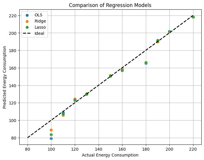
import pandas as pdimport numpy as npfrom sklearn.model_selection import train_test_splitfrom sklearn.linear_model import LinearRegression, Ridge, Lassofrom sklearn.metrics import mean_squared_error, r2_scoreimport matplotlib.pyplot as plt# Example data set: Predicting energy consumption based on temperature, humidity, and time of daydata = {'Temperature': [20, 25, 30, 15, 18, 22, 28, 32, 10, 12],'Humidity': [60, 70, 55, 65, 75, 62, 58, 45, 80, 72],'TimeOfDay': [10, 12, 14, 8, 9, 11, 13, 15, 7, 6],'EnergyConsumption': [150, 180, 200, 120, 130, 160, 190, 220, 100, 110]}df = pd.DataFrame(data)# Prepare the dataX = df[['Temperature', 'Humidity', 'TimeOfDay']]y = df['EnergyConsumption']X_train, X_test, y_train, y_test = train_test_split(X, y, test_size=0.2, random_state=42)# Define the modelsmodels = {'OLS': LinearRegression(),'Ridge': Ridge(alpha=1.0),'Lasso': Lasso(alpha=0.1)}results = {}predictions = pd.DataFrame({'Actual': y})# Train, evaluate, and predict for all modelsfor name, model in models.items(): model.fit(X_train, y_train) y_pred = model.predict(X) # Predict on all data predictions[name] = y_pred mse = mean_squared_error(y_test, model.predict(X_test)) # Evaluate on test set r2 = r2_score(y_test, model.predict(X_test)) results[name] = {'mse': mse, 'r2': r2, 'coefficients': model.coef_}# Results Tableresults_df = pd.DataFrame.from_dict(results, orient='index')print("\nModel Fit Results:")print(results_df)# Predictions Tableprint("\nPredictions:")print(predictions)# Scatterplotplt.figure(figsize=(8, 6))for name in models: plt.scatter(predictions['Actual'], predictions[name], label=name)plt.plot([80, 220], [80, 220], 'k--', lw=2, label='Ideal') # Add ideal lineplt.xlabel("Actual Energy Consumption")plt.ylabel("Predicted Energy Consumption")plt.title("Comparison of Regression Models")plt.legend()plt.grid(True)plt.show()
Summary of regularization behavior (python example):
Ridge regression shrinks coefficients towards zero, reducing their impact but not eliminating them entirely. It’s effective when many features are moderately important.
Lasso regression can shrink some coefficients to exactly zero, effectively performing feature selection. It’s useful when a few features are dominant.
OLS doesn’t have regularization, which can lead to overfitting if there are many features or the data is noisy.
Observe the coefficient plot to see how Ridge and Lasso shrink the coefficients compared to OLS. Experiment with different alpha values for Ridge and Lasso to see how it affects the results.